Take Home Exercise 1

Creating data visualisation beyond default

📖 Introduction

In Singapore, the residential property market is bifurcated into public and private sectors. The public housing sector serves households with a monthly income of up to S$14,000, aiming to offer affordable housing solutions to the broader community. In contrast, the private housing sector caters to households with incomes surpassing S$14,000.

For this analysis, we will leverage REALIS transaction data covering the period from 1st January 2023 to 31st March 2024. Our exploration will be conducted using ggplot2 and its associated extensions.

Setting the Scene

In this scenario, we assume the role of a graphical editor for a media company. We have been tasked with creating data visualizations to illuminate the private residential market and its sub-markets in Singapore for the first quarter of 2024.

Data Preparation

Load R Packages

pacman::p_load(tidyverse, haven,
               ggrepel, ggthemes,
               ggridges, ggdist,
               patchwork, scales,
               viridis, cowplot, 
               dplyr, plotly,
               tidyr, lubridate, 
               ggplot2, ggExtra)

Identify the missing values in the data set and removed any missing elements. ‘Type of Sale’ and ‘Property type’ has been converted to factor format. ‘Transacted Price ($)’ and ‘Area (SQFT)’ are converted to numeric data types. ‘Type of Sale’ has been group into three categories. ‘Sale Date’ has been converted to Date format.

The process had been repeated for all five data sets.

Import Data Sets

ds1 <- read_csv("data/ds1.csv")
ds2 <- read_csv("data/ds2.csv")
ds3 <- read_csv("data/ds3.csv")
ds4 <- read_csv("data/ds4.csv")
ds5 <- read_csv("data/ds5.csv")

Converting Data

prepare_dataset <- function(ds) {
  colSums(is.na(ds))
  ds <- na.omit(ds)
  
  ds$`Type of Sale` <- tolower(as.character(ds$`Type of Sale`))
  ds$`Type of Sale` <- ifelse(ds$`Type of Sale` %in% c("new sale", "resale"), ds$`Type of Sale`, "other")
  ds$`Type of Sale` <- as.factor(ds$`Type of Sale`)
  
  ds$`Property Type` <- as.factor(ds$`Property Type`)
  
  ds$`Transacted Price ($)` <- as.numeric(gsub("[^0-9.]", "", ds$`Transacted Price ($)`, perl = TRUE))
  ds$`Area (SQFT)` <- as.numeric(gsub("[^0-9.]", "", ds$`Area (SQFT)`, perl = TRUE))
  ds$`Unit Price ($ PSF)` <- as.numeric(gsub("[^0-9.]", "", ds$`Unit Price ($ PSF)`, perl = TRUE))
  
  return(ds)
}

# Apply the function to each dataset
ds1 <- prepare_dataset(ds1)
ds2 <- prepare_dataset(ds2)
ds3 <- prepare_dataset(ds3)
ds4 <- prepare_dataset(ds4)
ds5 <- prepare_dataset(ds5)

# Combine the datasets
combined_ds <- rbind(ds1, ds2, ds3, ds4, ds5)

Converting Dates

# Convert Sale Date to Date format
ds1$`Sale Date` <- dmy(ds1$`Sale Date`)
ds2$`Sale Date` <- dmy(ds2$`Sale Date`)
ds3$`Sale Date` <- dmy(ds3$`Sale Date`)
ds4$`Sale Date` <- dmy(ds4$`Sale Date`)
ds5$`Sale Date` <- dmy(ds5$`Sale Date`)

EDA

In this section, we will visualize the relationships between Property Types vs. Planning Region and Sale trend from Jan 2023 - Mar 2024.

Transactions by Regions and Property Type

Click to show code

transactions_heatmap <- combined_ds %>%
  group_by(`Planning Region`, `Property Type`) %>%
  summarise(Transactions = n()) %>%
  ungroup()

heatmap1 <- ggplot(transactions_heatmap, aes(x = `Planning Region`, y = `Property Type`, fill = Transactions)) +
  geom_tile() +
  labs(title = "Heatmap of Transactions by Region and Property Type",
       x = "Region",
       y = "Property Type") +
  scale_fill_viridis_c()

Transactions by Month

Click to show code

library(ggplot2)
library(dplyr)
library(lubridate)

# Combine all datasets into one dataframe
combined_ds <- bind_rows(ds1, ds2, ds3, ds4, ds5)

# Pre-process the combined dataset
combined_ds$`Sale Date` <- as.Date(combined_ds$`Sale Date`, format = "%Y-%m-%d")
combined_ds$Year <- year(combined_ds$`Sale Date`)
combined_ds$Month <- factor(format(combined_ds$`Sale Date`, "%b"), levels = month.abb)
combined_ds$`Number of Units` <- as.numeric(combined_ds$`Number of Units`)

# Summarize data to get total units sold by month and year
monthly_sales_combined <- combined_ds %>%
  group_by(Year, Month) %>%
  summarise(Units_Sold = sum(`Number of Units`, na.rm = TRUE)) %>%
  ungroup() %>%
  mutate(Month = factor(Month, levels = month.abb)) # Ensure months are in the correct order

# Create a single bar chart with month and year
barchart1 <- ggplot(monthly_sales_combined, aes(x = Month, y = Units_Sold, fill = as.factor(Year))) +
  geom_bar(stat = "identity", position = "dodge") +
  scale_x_discrete(drop = FALSE) + # Ensures all months are shown
  labs(title = "Total Number of Units Sold by Month and Year",
       x = "Month",
       y = "Number of Units Sold",
       fill = "Year") +
  theme_minimal() +
  theme(axis.text.x = element_text(angle = 45, hjust = 1),
        legend.position = "bottom")

Purchaser Address Indicator

Click to show code

percentage_data <- combined_ds %>%
  group_by(`Property Type`, `Purchaser Address Indicator`) %>%
  summarise(Count = n()) %>%
  group_by(`Property Type`) %>%
  mutate(Percentage = (Count / sum(Count)) * 100) %>%
  ungroup()
plot <- ggplot(percentage_data, aes(x = `Property Type`, y = Percentage, fill = `Purchaser Address Indicator`)) +
  geom_bar(stat = "identity", position = "stack") +
  geom_text(aes(label = sprintf("%.1f%%", Percentage)), 
            position = position_stack(vjust = 0.5), 
            size = 3, 
            color = "black") +
  labs(
    title = "Percentage of Purchaser Address Indicator by Property Type",
    x = "Property Type",
    y = "Percentage (%)",
    fill = "Purchaser Address Indicator"
  ) +
  theme_minimal() +
  theme(
    axis.text.x = element_text(angle = 45, hjust = 1),
    legend.position = "top"
  )

Sale Categories vs. Property Types

Click to show code

counts <- table(combined_ds$`Type of Sale`, combined_ds$`Property Type`)
percentages <- prop.table(counts, margin = 1) * 100 

df_percentages <- as.data.frame(as.table(percentages))

barchart <- ggplot(df_percentages, aes(x = Var1, y = Freq, fill = Var2)) +
  geom_bar(stat = "identity", position = "dodge") +
  geom_text(aes(label = sprintf("%.1f%%", Freq)), position = position_dodge(width = 0.9), vjust = -0.5, size = 2) +  
  labs(title = "Comparing Property Types Across Sale Categories",
       x = "Sale Categories",
       y = "Percentage (%)", 
       fill = "Property Type") +
  scale_fill_brewer(palette = "Set3") +
  theme_minimal() +
  theme(legend.position = "top") 

Click to show code

# Adjust text size for the bar chart
barchart1 <- barchart1 + theme(
  plot.title = element_text(size = 8),      # Adjust title size
  axis.title = element_text(size = 8),       # Adjust axis titles size
  axis.text.x = element_text(size = 6, angle = 45, hjust = 1), # Adjust x axis text size
  axis.text.y = element_text(size = 6),      # Adjust y axis text size
  legend.text = element_text(size = 6)       # Adjust legend text size
)

# Adjust text size for the heatmap
# Adjust the heatmap to move the legend to the bottom
heatmap1 <- heatmap1 + theme(
  plot.title = element_text(size = 8), 
  axis.text.x = element_text(size = 6, angle = 45, hjust = 1), # Adjust x axis text size
  axis.text.y = element_text(size = 6), 
  legend.position = "bottom",
  legend.text = element_text(size = 6, angle = 45, hjust = 1),       # Adjust legend text size if necessary
  legend.title = element_text(size = 6)       # Adjust legend title size if necessary
)

# Adjusting theme settings for barchart
barchart <- barchart + theme(
  plot.title = element_text(size = 8),  # Smaller plot title
  axis.title = element_text(size = 8),   # Smaller axis titles
  axis.text = element_text(size = 6),    # Smaller axis text
  legend.text = element_text(size = 6),  # Smaller legend text
  legend.title = element_text(size = 6)  # Smaller legend title
)

# Adjusting theme settings for plot
plot <- plot + theme(
  plot.title = element_text(size = 8),
  axis.title = element_text(size = 8),
  axis.text = element_text(size = 6),
  legend.text = element_text(size = 6),
  legend.title = element_text(size = 8)
)

# Now combine the plots using patchwork
combined_plot2 <- (barchart | plot) +
  plot_layout(widths = c(1, 1))  # Adjust the relative widths if necessary

# Print the combined plot
print(combined_plot2)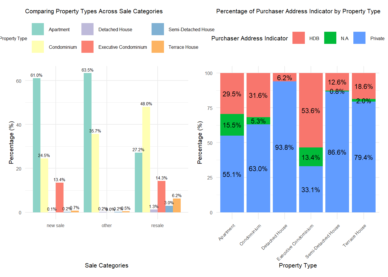

According to REALIS data dictionary, ‘Purchaser Address Indicator’ refers to the type of residence (either HDB flat or private property) associated with the purchaser’s address as indicated in the caveat. It doesn’t necessarily imply ownership but rather reflects the type of housing the purchaser resides in. If this information is unavailable, it’s marked as ‘N.A’.

combined_plot <- barchart1 + heatmap1 + 
  plot_layout(widths = c(0.1, 0.1)) # Adjust the width ratio as needed
print(combined_plot)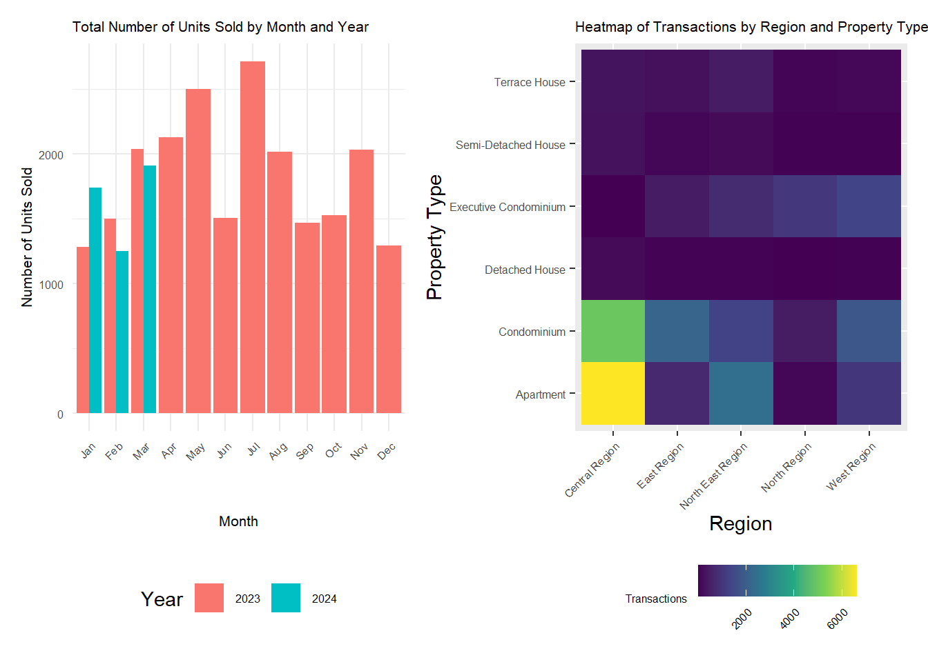

combined_plot2 <- (barchart | plot) +
  plot_layout(widths = c(1, 1.5)) 
print(combined_plot2)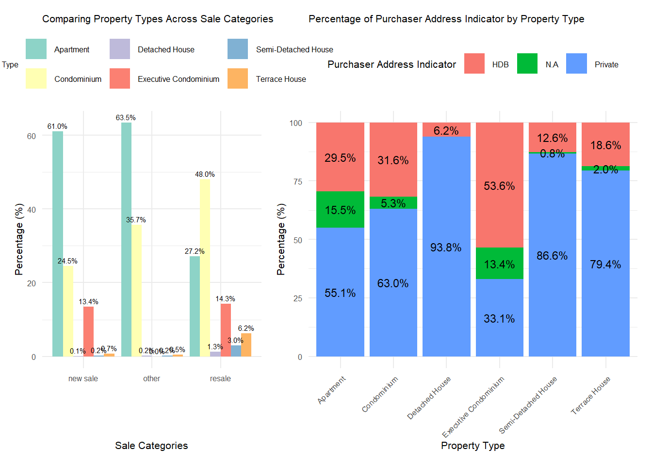

📈 Insight:

• Private property sales surge in Jul 2023 due to several big launches on the market and developers sold 1412 units in July compared to 278 in June. Read more.
  
• Central Region Apartments are the most sought after in the market according to the heatmap, followed by condominiums.
  
• In the new sale market, apartments represent 61% of sales, while condominiums make up 24.5%. In contrast, the resale market sees condominiums accounting for 48% and apartments at 27.2%. Detached, semi-detached, and terrace houses are less prevalent in both markets. This is attributed to land scarcity and high construction costs imposed by the Singapore government. Furthermore, many property owners retain these types of properties due to their freehold tenure.
  
• It’s notable that a significant majority of private property buyers (presumably those residing in these properties) live in private residences. Interestingly, executive condominiums have the highest proportion of purchasers with HDB addresses, accounting for 53.6%. This could be attributed to the attractive rental yields in Singapore. Consequently, more residents might be purchasing executive condominiums primarily as investment properties.
  

EDA 2

We analyzed unit price ($PSF) across Singapore’s planning regions for 2023, using four quarterly charts to visualize regional price variations. The Central Region consistently showed the highest median PSF, indicating its premium status. In contrast, the North East and East Regions maintained stable PSF values, balancing affordability with location.

Click to show code

q4 <- ggplot(ds2, aes(x = `Planning Region`, y = `Unit Price ($ PSF)`)) +
  geom_boxplot() +
  labs(title = "Price per Square Foot by Planning Region - Oct 23 - Dec 23",
       x = "Planning Region",
       y = "Unit Price ($ PSF)") +
  theme(text = element_text(size = 6)) 

# Price per Square Foot by Planning Region in DS3
q3 <- ggplot(ds3, aes(x = `Planning Region`, y = `Unit Price ($ PSF)`)) +
  geom_boxplot() +
  labs(title = "Price per Square Foot by Planning Region - Jul 23 - Sep 23",
       x = "Planning Region",
       y = "Unit Price ($ PSF)") +
  theme(text = element_text(size = 6)) 

# Price per Square Foot by Planning Region in DS4
q2 <- ggplot(ds4, aes(x = `Planning Region`, y = `Unit Price ($ PSF)`)) +
  geom_boxplot() +
  labs(title = "Price per Square Foot by Planning Region - Apr 23 - Jun 23",
       x = "Planning Region",
       y = "Unit Price ($ PSF)") +
  theme(text = element_text(size = 6)) 

# Price per Square Foot by Planning Region in DS5
q1 <- ggplot(ds5, aes(x = `Planning Region`, y = `Unit Price ($ PSF)`)) +
  geom_boxplot() +
  labs(title = "Price per Square Foot by Planning Region - Jan 23 - Mar 23",
       x = "Planning Region",
       y = "Unit Price ($ PSF)") +
  theme(text = element_text(size = 6)) 

combined_plot <- wrap_plots(q1, q2, q3, q4)
combined_plot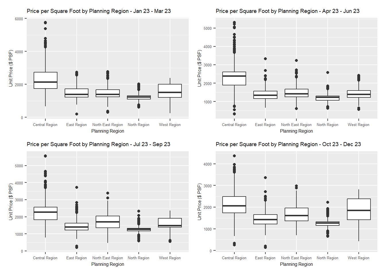

Click to show code

combined_ds <- bind_rows(
  ds1 %>% mutate(Data_Source = "data/ds1.csv"),
  ds2 %>% mutate(Data_Source = "data/ds2.csv"),
  ds3 %>% mutate(Data_Source = "data/ds3.csv"),
  ds4 %>% mutate(Data_Source = "data/ds4.csv"),
  ds5 %>% mutate(Data_Source = "data/ds5.csv"),
)

summary_stats <- combined_ds %>%
  group_by(`Planning Region`) %>%
  summarise(
    median_PSF = median(`Unit Price ($ PSF)`, na.rm = TRUE),
    lower_quartile = quantile(`Unit Price ($ PSF)`, 0.25, na.rm = TRUE),
    upper_quartile = quantile(`Unit Price ($ PSF)`, 0.75, na.rm = TRUE)
  )

p <- ggplot(combined_ds, aes(x = `Planning Region`, y = `Unit Price ($ PSF)`)) +
  geom_boxplot() +
  stat_summary(
    fun = median,
    geom = "point",
    shape = 23,
    size = 3,
    color = "blue",
    position = position_dodge(width = 0.75)
  ) +
  labs(
    title = "Distribution of Price per Square Foot by Planning Region - 2023 Q1-Q4",
    x = "Planning Region",
    y = "Unit Price ($ PSF)"
  ) +
  theme_minimal() +
  theme(axis.text.x = element_text(angle = 45, hjust = 1))

p_plotly <- ggplotly(p, tooltip = c("Planning Region", "y", "Data_Source", "median_PSF", "lower_quartile", "upper_quartile"))

p_plotly <- plotly::ggplotly(p, tooltip = c("Planning Region", "y", "Data_Source", "median_PSF", "lower_quartile", "upper_quartile"))

p_plotly

📈 Insight:
Each region in Singapore offers a unique property market landscape catering to different buyer preferences and budgets.
The Central Region stands out as a high-end market, while the East offers premium properties at better values.
The North East and North Regions provide a mix of affordability and mid-range options, whereas the West Region offers diversity without extreme price outliers.

EDA 3

library(viridis)

ggplot(combined_ds, aes(x = `Unit Price ($ PSF)`, y = `Planning Region`, fill = `Planning Region`)) +
  geom_density_ridges(scale = 3) +
  scale_fill_viridis(discrete = TRUE) +
  labs(title = "Unit Price ($ PSF) Distribution by Planning Region",
       x = "Unit Price ($ PSF)",
       y = "Planning Region") +
  theme_ridges()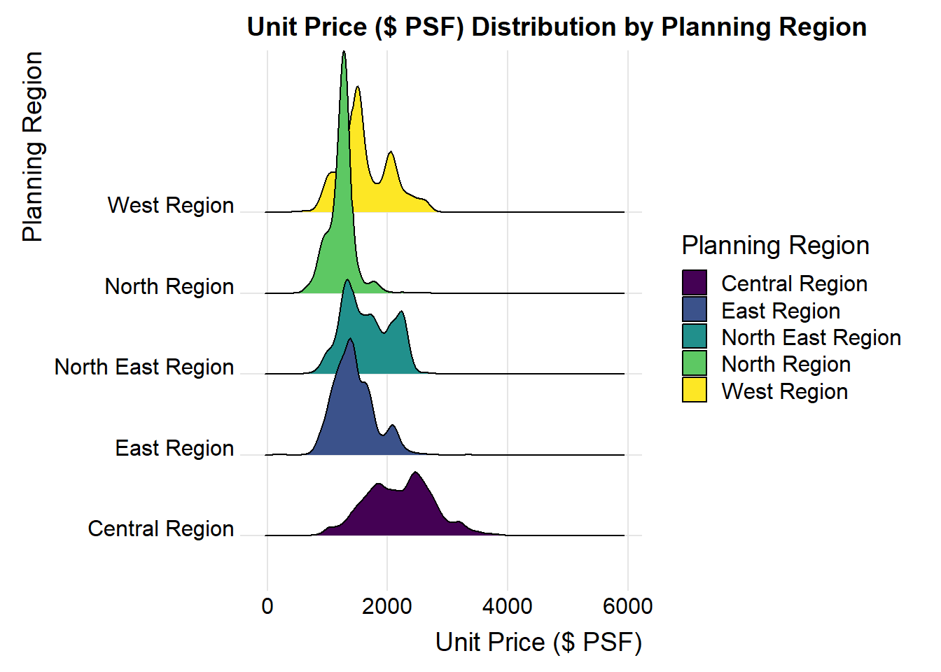

📈 Insight:
- The Central Region’s peak is the most pronounced and shifted towards the high, indicating that there is a high concentration of properties with higher unit prices.
- The East Region’s pea is lower and more towards the middle of the x-axis compared to the Central Region. This implies that while the East Region has properties with moderate unit prices, it does not reach as high of a price point as frequently as the Central Region.
- North East and North Regions peaks are less sharp and positioned towards the lower end of the price scale, suggesting a more affordable housing options and a wider distribution of unit prices. North Region appears to have a slightly broader distribution than North East.
- West Region has the lowest peak among all the regions and is positioned towards the far left of the plot. This indicates that the West Region is the most affordable in Singapore.