In Class Exercise 4

Getting Started

pacman::p_load(tidyverse, ggstatsplot)

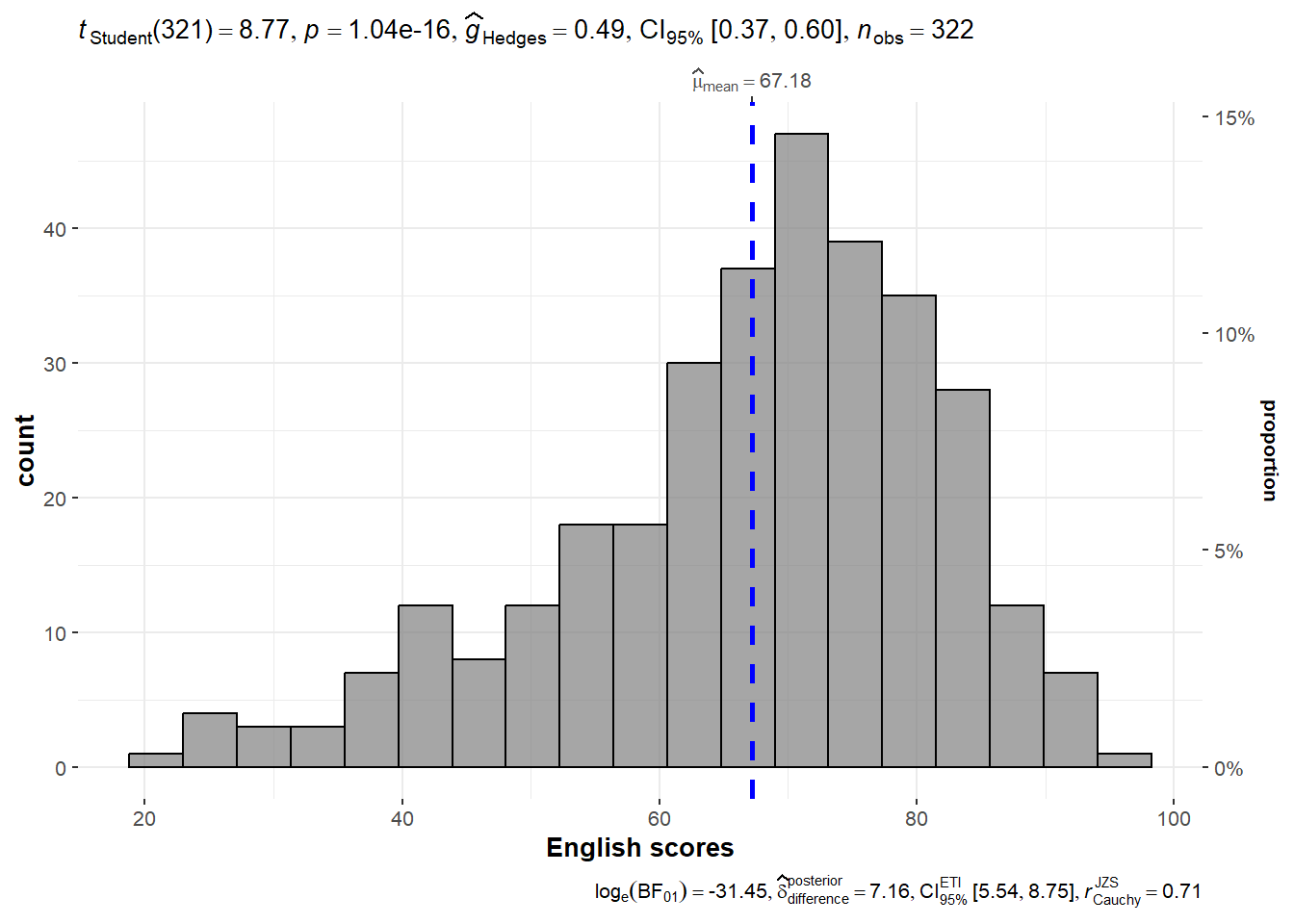
exam <- read_csv("data/Exam_data.csv")

set.seed(1234)

gghistostats(
  data = exam,
  x = ENGLISH, 
  type = 'parametric',
  test.value = 60, 
  bin.args = list(color = "black",
                  fill = "grey50",
                  alpha = 0.7), 
  normal.curve = FALSE,
  normal.curve.args = list(linewidth 
= 2), 
  xlab = "English scores"
)

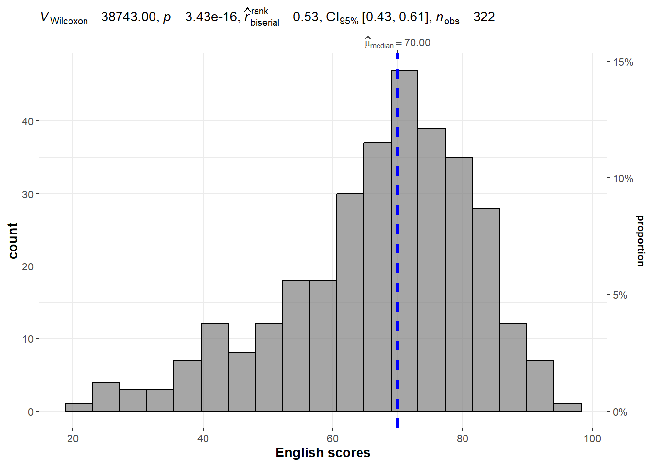
gghistostats(
  data = exam,
  x = ENGLISH, 
  type = 'np',
  test.value = 60, 
  bin.args = list(color = "black",
                  fill = "grey50",
                  alpha = 0.7), 
  normal.curve = FALSE,
  normal.curve.args = list(linewidth 
= 2), 
    xlab = "English scores"
)

p <- gghistostats(
  data = exam,
  x = ENGLISH, 
  type = 'np',
  test.value = 60, 
  bin.args = list(color = "black",
                  fill = "grey50",
                  alpha = 0.7), 
  normal.curve = FALSE,
  normal.curve.args = list(linewidth 
= 2), 
    xlab = "English scores"
)

extract_stats(p)

$subtitle_data
# A tibble: 1 × 12
  statistic  p.value method                    alternative effectsize       
      <dbl>    <dbl> <chr>                     <chr>       <chr>            
1     38743 3.43e-16 Wilcoxon signed rank test two.sided   r (rank biserial)
  estimate conf.level conf.low conf.high conf.method n.obs expression
     <dbl>      <dbl>    <dbl>     <dbl> <chr>       <int> <list>    
1    0.528       0.95    0.430     0.613 normal        322 <language>

$caption_data
NULL

$pairwise_comparisons_data
NULL

$descriptive_data
NULL

$one_sample_data
NULL

$tidy_data
NULL

$glance_data
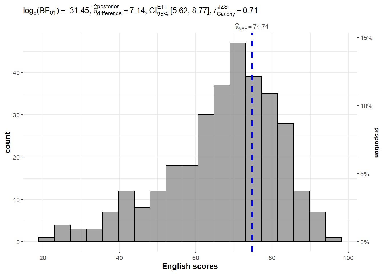
NULL

  gghistostats(
  data = exam,
  x = ENGLISH, 
  type = 'bayes',
  test.value = 60, 
  bin.args = list(color = "black",
                  fill = "grey50",
                  alpha = 0.7), 
  normal.curve = FALSE,
  normal.curve.args = list(linewidth = 2), 
  xlab = "English scores"
)

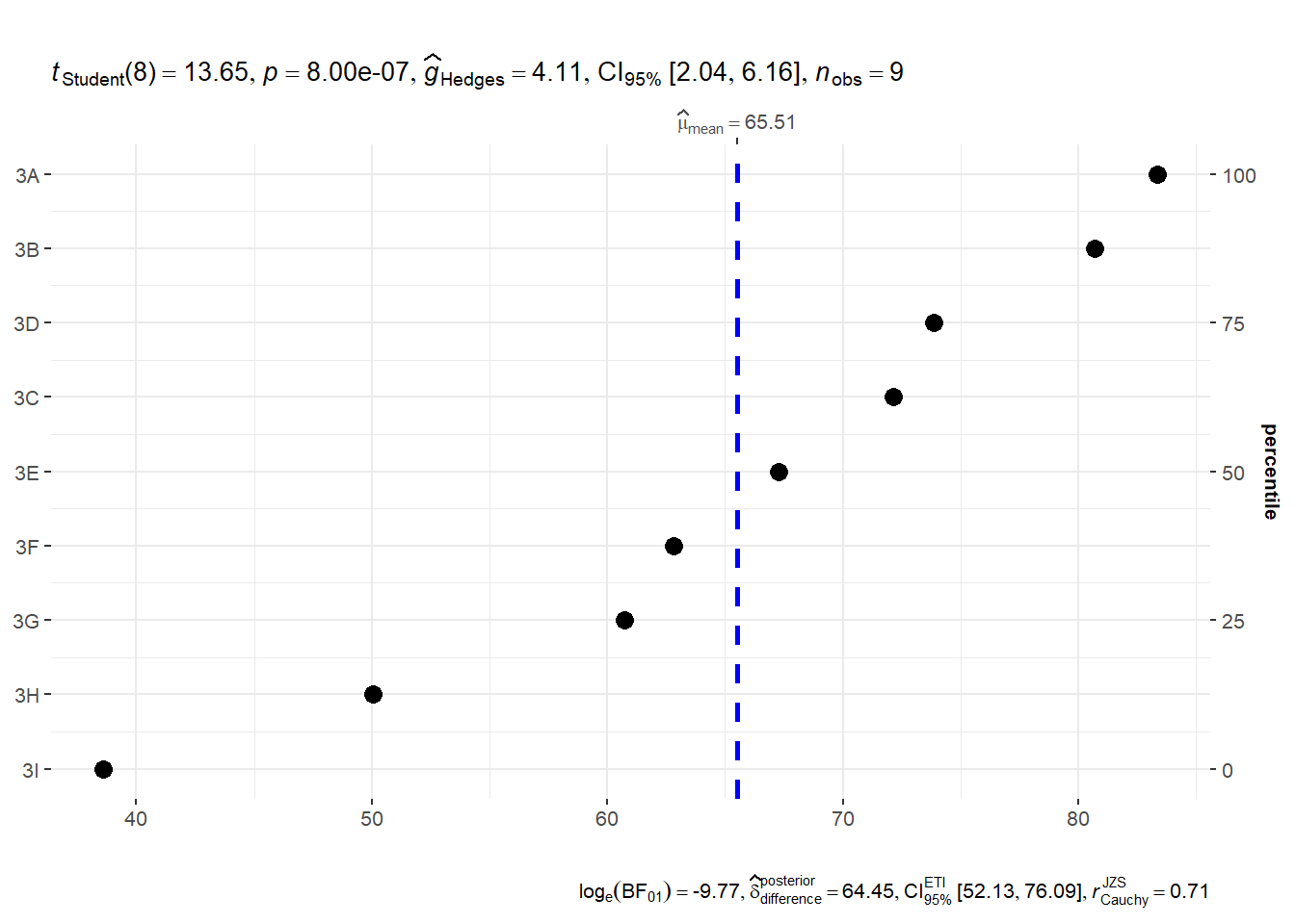
ggdotplotstats(
  data = exam,
  x = ENGLISH, 
  y = CLASS,
  title = "",
  xlab = ""
  
)

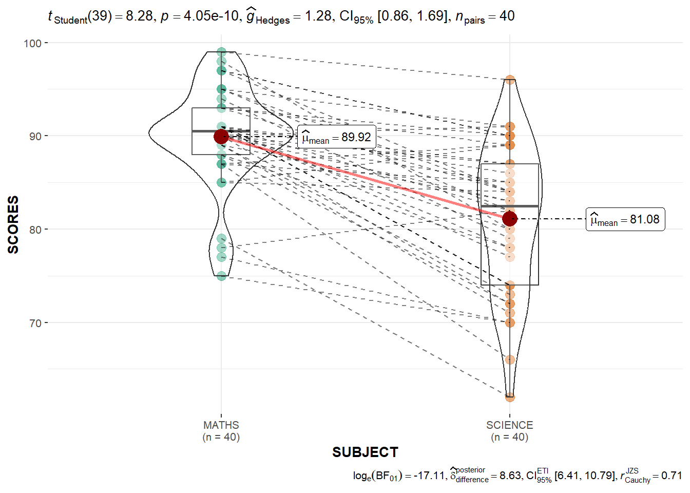
exam_long <- exam %>%
   pivot_longer(
     cols = ENGLISH:SCIENCE,
     names_to = "SUBJECT",
     values_to = "SCORES") %>%
  filter(CLASS =="3A")

ggwithinstats(
    data = filter(exam_long,
                SUBJECT %in%
                  c("MATHS", "SCIENCE")),
  x    = SUBJECT,
  y    = SCORES,
  type = "p"
)

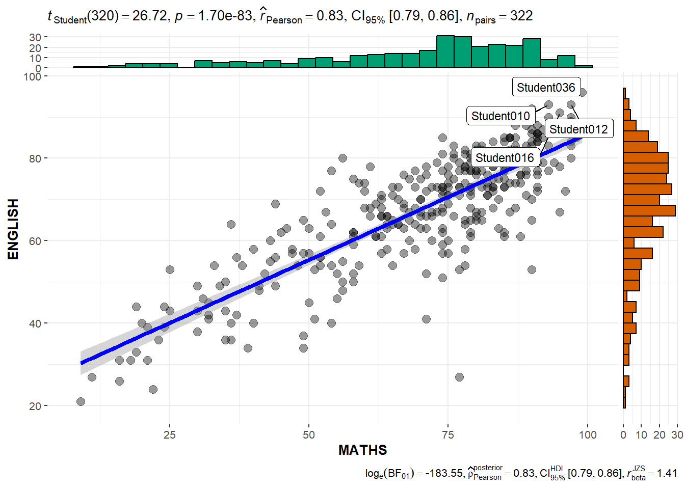
ggscatterstats(
  data = exam,
  x = MATHS,
  y = ENGLISH, 
  marginal = TRUE, 
  label.var = ID,
  label.expression = ENGLISH >90 & MATHS  > 90,
)